Details of intersection of radar grid with CML paths
This notebook shows the details of how the intersection of a grid and lines is done. The typicall use case is doing this for gridded radar rainfall data and CML paths, but it would work the same for gridded satellite data and SMLs.
[1]:
import matplotlib.pyplot as plt
import xarray as xr

import poligrain as plg
Load example data
[2]:
ds_cmls = xr.open_dataset("../../tests/test_data/openMRG_CML_180minutes.nc")
[3]:
ds_radar = xr.open_dataset("../../tests/test_data/openMRG_Radar_180minutes.nc")
Calculate intersection weights
Note that the intersection weights are stored as sparse.arrays in a xarray.DataArray because the matrix of intersection weights for each CMLs, based on the radar grid, contains mostly zeros. Hence, we can save a lot of space. For large CML networks this is crucial because storing thousands of intersection weight matrices, one for each CML, easily eats up 10s of GBs of memory.
Note that this calculation is fairly fast, i.e. approx. 2 seconds for 500 CMLs.
[4]:
%%time
da_intersect_weights = plg.spatial.calc_sparse_intersect_weights_for_several_cmls(
    x1_line=ds_cmls.site_0_lon.values,
    y1_line=ds_cmls.site_0_lat.values,
    x2_line=ds_cmls.site_1_lon.values,
    y2_line=ds_cmls.site_1_lat.values,
    cml_id=ds_cmls.cml_id.values,
    x_grid=ds_radar.lon.values,
    y_grid=ds_radar.lat.values,
    grid_point_location="center",
)
CPU times: user 585 ms, sys: 10.4 ms, total: 595 ms
Wall time: 609 ms
[5]:
da_intersect_weights.isel(cml_id=0)
[5]:
<xarray.DataArray (y: 48, x: 37)>
<COO: shape=(48, 37), dtype=float64, nnz=1, fill_value=0.0>
Coordinates:
    x_grid   (y, x) float64 11.41 11.45 11.48 11.51 ... 12.56 12.59 12.62 12.66
    y_grid   (y, x) float64 58.04 58.04 58.04 58.04 ... 57.23 57.23 57.23 57.23
    cml_id   int64 10001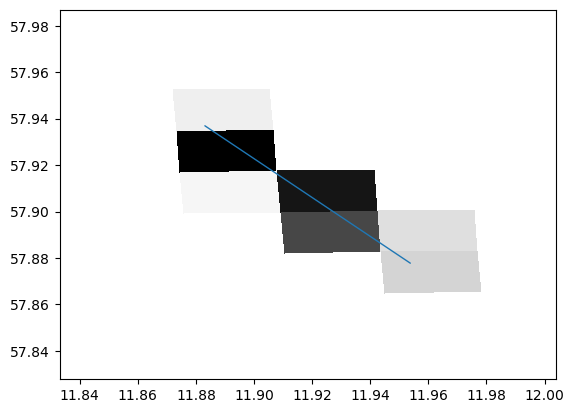
Dimensions without coordinates: y, xPlot intersection weights and CML path
Darker colors indicate a higher intersection weight.
[6]:
i = 10202
cml = ds_cmls.sel(cml_id=i)
plt.pcolormesh(
    ds_radar.lon.values,
    ds_radar.lat.values,
    da_intersect_weights.sel(cml_id=i).to_numpy(),
    cmap="Greys",
)

plg.plot_map.plot_lines(ds_cmls.sel(cml_id=i), ax=plt.gca())

plt.ylim(
    min(cml.site_0_lat.values, cml.site_1_lat.values) - 0.05,
    max(cml.site_0_lat.values, cml.site_1_lat.values) + 0.05,
)
plt.xlim(
    min(cml.site_0_lon.values, cml.site_1_lon.values) - 0.05,
    max(cml.site_0_lon.values, cml.site_1_lon.values) + 0.05,
)
[6]:
(11.833089999999999, 12.00378)
Get time series of radar rainfall along CML for each CML
This is internally done via a sparase.tensordot product, which is very fast, given that the intersection weights are also stored as sparse.arrays. The convenience funtion from poligrain used here, also takes care of adding the correct coordinates to the xarray.DataArray that is returned.
Note that this calculation is very fast and can be done with a large number of CMLs and a much longer period of radar data.
[7]:
%%time

da_radar_along_cmls = plg.spatial.get_grid_time_series_at_intersections(
    grid_data=ds_radar.rainfall_amount,
    intersect_weights=da_intersect_weights,
)
CPU times: user 320 ms, sys: 7.6 ms, total: 327 ms
Wall time: 328 ms
[8]:
da_radar_along_cmls
[8]:
<xarray.DataArray (time: 36, cml_id: 364)>
array([[5.45577289e-02, 1.29376820e-01, 5.15058173e-02, ...,
        4.86375435e-04, 2.60098642e-01, 7.85087184e-02],
       [4.86246270e-02, 4.86246443e-04, 4.86246236e-04, ...,
        2.68530211e-02, 4.86150392e-04, 4.86179854e-04],
       [4.86246236e-04, 4.86246443e-04, 4.86246236e-04, ...,
        4.86375435e-04, 4.86150392e-04, 4.86179854e-04],
       ...,
       [1.22139538e-02, 4.86246443e-04, 1.15307163e-01, ...,
        4.86375435e-04, 5.55353035e-02, 5.13666248e-02],
       [2.17198235e-01, 3.44236153e-01, 6.86841139e-01, ...,
        4.86375435e-04, 7.50213222e-02, 2.72055320e-01],
       [1.08856978e-02, 3.06800794e-01, 3.06800653e-02, ...,
        3.92748636e-02, 1.30498263e-01, 5.51433563e-02]])
Coordinates:
  * time     (time) datetime64[ns] 2015-08-27T00:20:00 ... 2015-08-27T03:15:00
* cml_id (cml_id) int64 10001 10002 10003 10004 ... 10361 10362 10363 10364[9]:
# The following show how you write the data to a NetCDF to use it somewhere else.
#
# da_radar_along_cmls.to_dataset(name='rainfall_amount').to_netcdf(
#    '..poligrain/tests/test_data/openMRG_example_path_averaged_reference_data.nc',
#    encoding={'rainfall_amount': {'zlib': True}}
# )
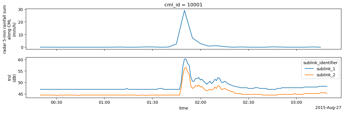
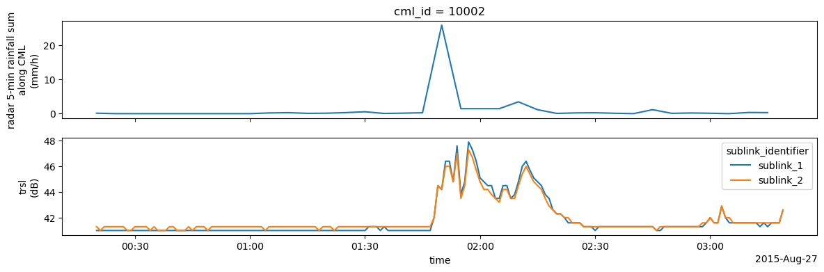
Plot radar along CML vs. TL
We set non-meaningfull RSL and TSL values to NaN.
Here we only plot radar rain rates vs TL. For plotting CML-derived rain rates, processing has to be done first. But the comparison with TRSL already shows the good match between CML attenuation data and rainfall data.
[10]:
ds_cmls["tsl"] = ds_cmls.tsl.where(ds_cmls.tsl < 100)
ds_cmls["rsl"] = ds_cmls.rsl.where(ds_cmls.rsl > -99)

ds_cmls["trsl"] = ds_cmls.tsl - ds_cmls.rsl
[11]:
for i in range(5):
    fig, axs = plt.subplots(2, 1, figsize=(14, 4), sharex=True)
    da_radar_along_cmls.isel(cml_id=i).plot(ax=axs[0])
    ds_cmls.isel(cml_id=i).trsl.plot.line(x="time", ax=axs[1])
    axs[0].set_xlabel("")
    axs[0].set_ylabel("radar 5-min rainfall sum\nalong CML\n(mm/h)")
    axs[1].set_title("")
    axs[1].set_ylabel("trsl\n(dB)")


Plot radar map and the results of the grid intersection
Here the 3 hour rainfall sum is shown for the radar rainfall field and the path integrated radar rainfall along each CML.
The path integrated radar rainfall on the bottom right plot can be used to compare the CML rainfall estimates to the radar rainfall.
[12]:
ds_cmls["radar_along_cmls"] = da_radar_along_cmls

fig, ax = plt.subplots(1, 2, figsize=(10, 4), sharey=True, sharex=True)

(ds_radar.rainfall_amount.sum(dim="time") / 12).plot(
    x="lon", y="lat", ax=ax[0], cmap="YlGnBu", vmin=0, vmax=9
)
plg.plot_map.plot_lines(ds_cmls, ax=ax[0], line_color="grey", line_width=0.5)

da_ralong = (
    ds_cmls.radar_along_cmls.sum(dim="time") / 12
)  # from intensity (mm/h) to amount (mm)
lines_radar_along_cml = da_ralong.plg.plot_cmls(
    pad_width=0.5, cmap="YlGnBu", ax=ax[1], vmin=0, vmax=9
)
plt.colorbar(lines_radar_along_cml, label="rainfall amount in mm")

plt.tight_layout()
